MySql InnoDB Indexes for Developers
This article aims to be a high level reference for developers who just want to use Mysql InnoDB indexes effectively. While you can read this from top to bottom, I’ve also included a table of contents if you want to jump to a particular topic.
Contents
Index Structure
Indexes are constructed from a B+tree structure. Understanding this structure is key to gaining an intuitive reasoning for how queries will perform using different indexes. Both the PRIMARY index and secondary indexes have a similar tree structure, differing only in what data is stored on the leaves of the tree.
Primary Index Structure & Paging
Looking at the structure of a PRIMARY index first, we see that the full row is stored in each leaf of the tree, and each leaf is ordered sequentially on the disk:
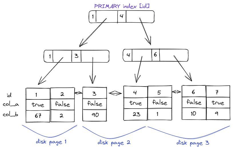
Knowing this structure allows us to design more performant primary indexes. Loading a page from disk into memory is typically the slowest part about making a primary index lookup, so reducing the number of page loads can greatly improve the performance of our primary index queries. One of the best ways we can reduce the number of page loads is to design the primary index with data locality in mind. That is: data which is often read at the same time, is generally located in the same disk pages.
For example, imagine a multi-tenant blogging application that almost always bulwarks queries by a specific blog: SELECT * FROM posts WHERE blog_id=10 AND .... Ideally we’d like for this table to have all the posts where blog_id = 10 stored sequentially in the primary index.
First lets look at the common practice of using a basic primary index on a single auto_incremented [id] column. In this design, we see a structure where rows are stored in disk pages in the order they were created. The diagram below illistrates this (ID integer, colour coded by blog)
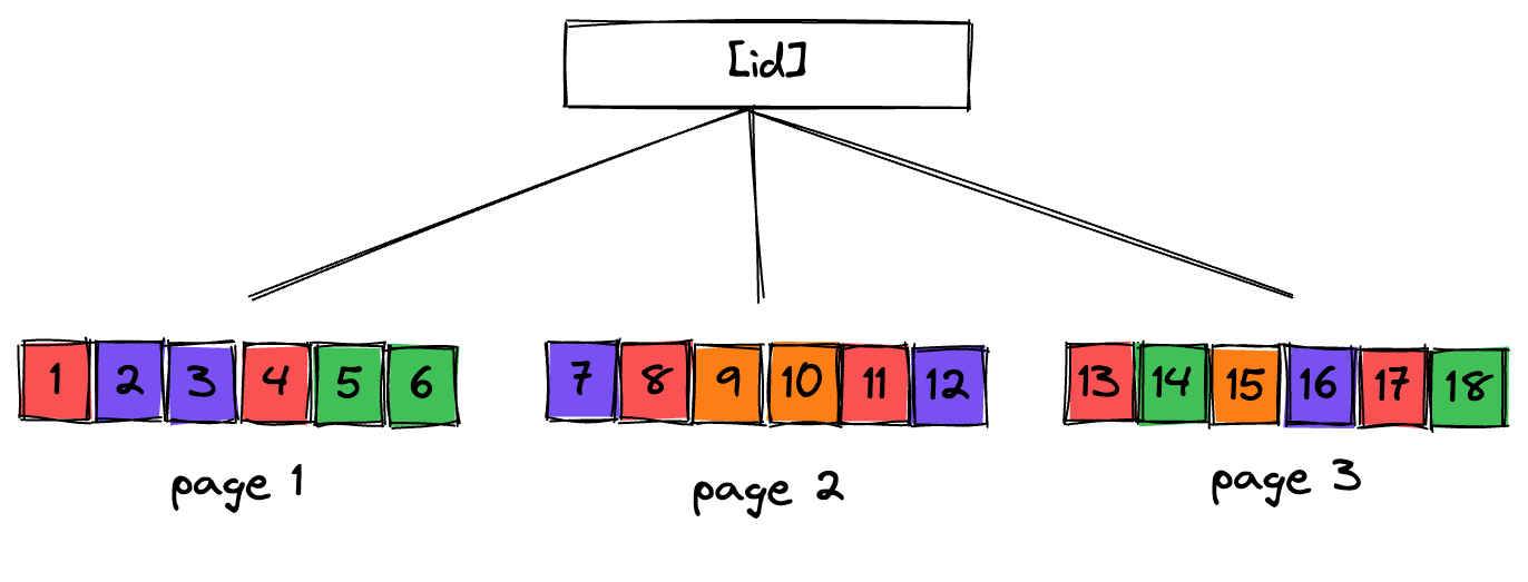
In this design, the number of page loads could be as high as 1 page per blog post. In fact this is likely the case for any blogging platform at scale.
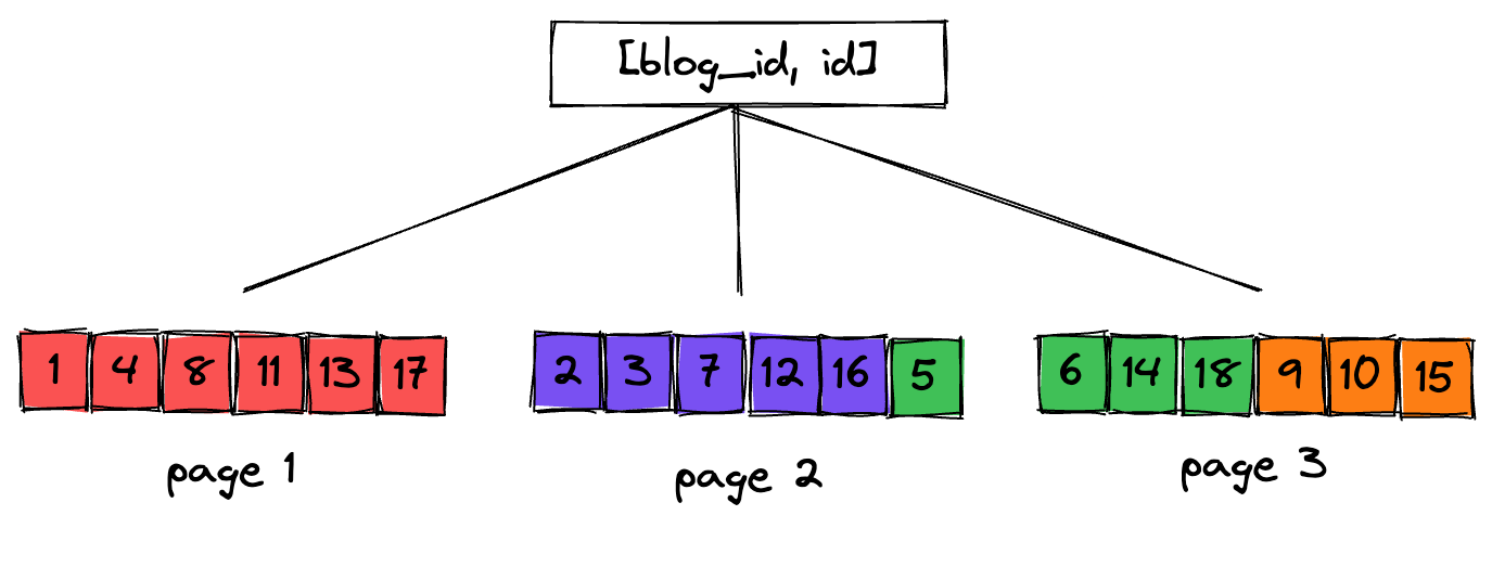
By instead using a composite primary key, this table can be made much more efficient given its access pattern. In the below diagram I show the same data, but instead stored in a composite primary index of [blog_id, id]. This means rows are stored on disk sorted first by blog_id, and then by id. When the data is stored in this manner, our query for SELECT * FROM posts WHERE blog_id=10 is much likely to load less pages from disk.
Secondary Index Structure
Secondary indexes have a similar structure to that of primary indexes. However, instead of storing the full row in the leaves of the tree, only the primary index value is stored.
For example, if our blogging platform’s Posts table has a Primary Index [id], and we build a Secondary Index on [user_id], we will get a structure like this:
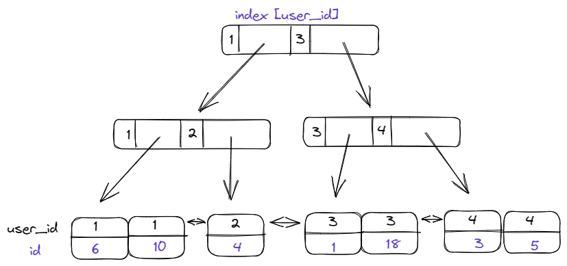
By navigating this tree for a particular user_id, we will be given the set of post IDs for that user. In the above diagram, if we searched for WHERE user_id=3, we will receive an answer of ids => [1, 18].
Now, if ID is all we were interested in (SELECT id WHERE user_id=3), then we’re done, great!
However, if additional columns are required (SELECT *), then mysql must now also traverse the primary index for each selected row to actually load the required data (because the full row data is stored in the primary index only). We can use this knowledge to our advantage: by only selecting columns available in the secondary index, mysql can skip the extra primary index lookup step.
If you’ve ever heard someone say something like: “an index on [user_id] is really an implied composite index with ID in the last position ([user_id, id])”, this is why.
Composite Index Structure
When multiple columns are specified in a compound index, we get a structure composed of nested B+trees. This is where the ordering of columns within an index definition becomes relevant. The root of the tree is defined by the first column in the index definition, the second level tree would be the second column in the index definition, and so on.
The below diagram is the structure of a composite index [blog_id, created_at] (with the implied id column on the end):
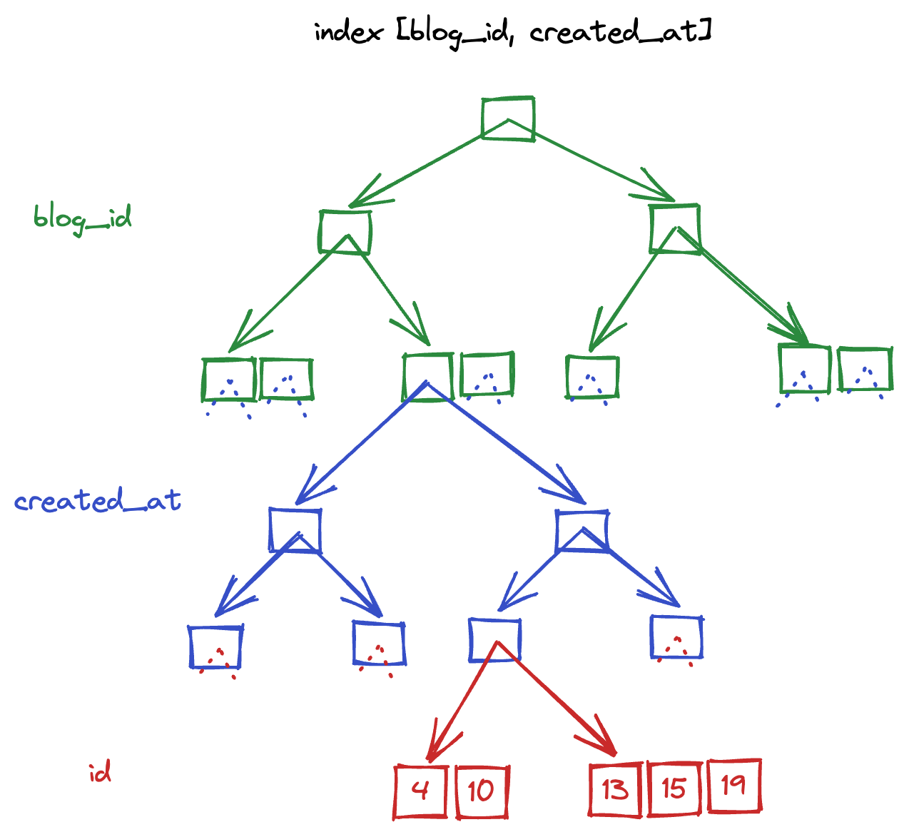
The main thing to notice here is that each leaf of the top-most tree has another tree embedded within it. So while there is a single tree representing the first column (blog_id), there are multiple trees representing the second column (created_at), one per value of blog_id.
In other words, while there is a single entry point to the blog_id portion of the tree, there are N entry points to the created_at portion of the tree. As we will see in the following sections, this introduces an asymmetry that brings meaning to the order in which columns are defined in an index (ie [blog_id, created_at] != [created_at, blog_id])
Index Navigation
We’ll now look at how mysql navigates these indexes given various query structures, which should help give an intuitive understanding for why Mysql performance will vary.
ref-type queries
With this tree-based model in place, we can see that to efficiently use an index like this we must navigate the tree in the order that the index is defined. If our query does not specify a value for all columns in an index, this is ok as long as the values we do provide are at the top of the tree.
I’ve illustrated below two examples of the “happy path” for navigating a [blog_id, user_id] index. In the first, we have provided a filter on both blog_id and user_id, which allows for mysql to fully navigate the tree to the leaves. In the second, we only provide a filter on blog_id, but because this is the first column in the index mysql is still able to efficiently select all the rows that meet this criteria. Remember: rows in this index are stored on disk ordered by blog_id, user_id. Therefore if mysql can find the first row where the blog_id condition matches (ie the left-most leaf), it knows that all the other relevant rows will be directly sequential. Once mysql finds a row with a different blog_id, the row scanning is halted.
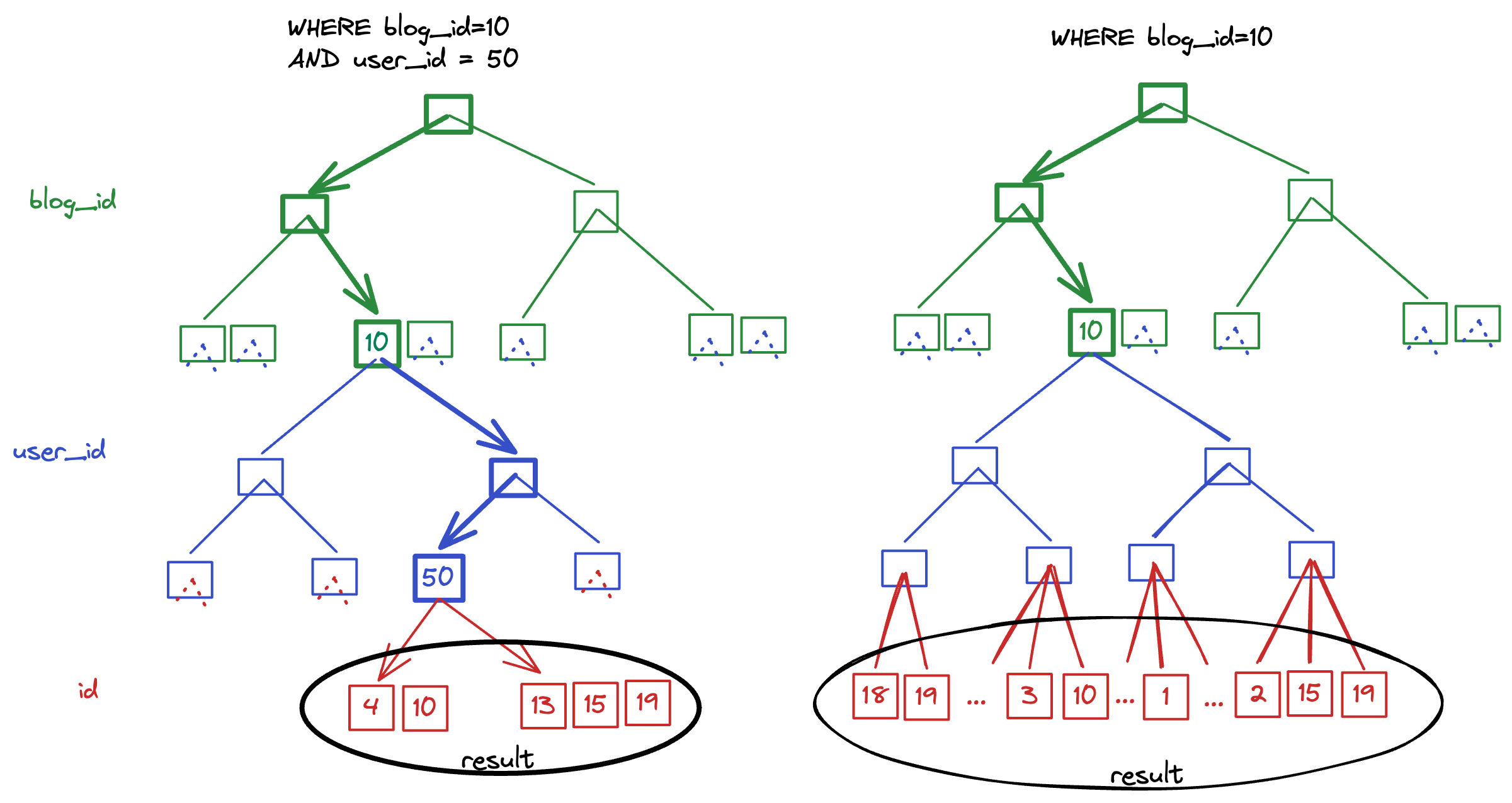
💡 Notice how the ordering of the rows appears to change depending on how far mysql navigates the tree. Rows in an index are always stored in the same ordering scheme as the index itself. That is to say that a [blog_id, user_id] index will naturally store rows in blog_id, user_id, id ordering. However, as we navigate further into the tree the ordering appears to “simplify”. If we are selecting rows for a specific blog=10 and user_id=50 then the rows appear to be ordered by id, because they all share the same values for both blog_id and user_id!
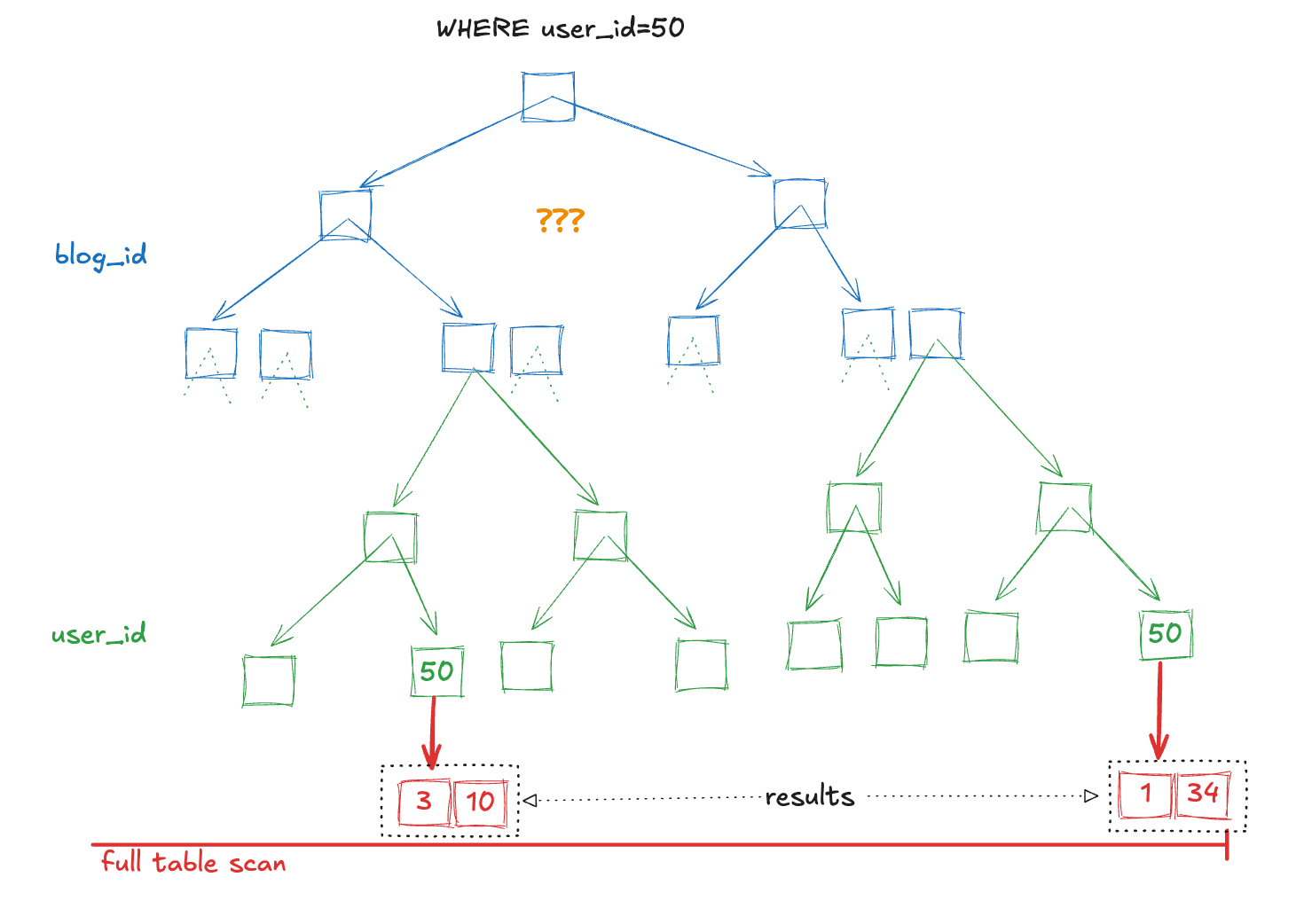
Let’s also quickly look at a situation where the same [blog_id, user_id] index is not able to help us. This time we will only filter by user_id. Notice that because the user we are looking for may be in any of the N sub-trees, there is no clear path to navigate this index. In this situation, mysql will opt to scan the full table rather than use our index.
range-type queries
The range-type lookup happens when a query selects multiple values for an indexed column. There are a couple ways a query could end up in this scenario, and I like to classify them into two sub-categories (note that these are my personal names, and mysql EXPLAIN does not differentiate these two):
- True Range Queries
- Finite Range Queries
Lets look at each one seperately.
True Range Queries
True range queries are those that select a potentially unbounded number of values for a column. The main ways you’ll run into these types of queries are:
WHERE updated_at >= XWHERE user_id != X
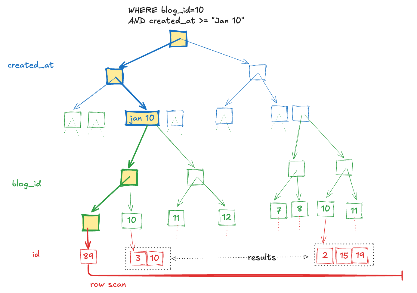
For these types of queries, mysql is going to navigate the index to find the boundaries of the range(s), then leverage the natural sorting order of rows to scan and select rows. Below I’ve included examples of “happy path” True Range queries.
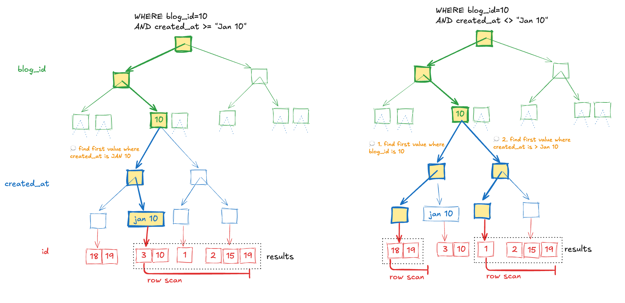
💡 Notice that because multiple branches of the created_at portion of the index are used, the ordering of the results is created_at, id. Sorting a range query by the primary index requires an extra filesort!
Let’s also take a quick look at one of the main limitations of true-range type queries: Once a part of the index is used for a range, no further parts of the index can be used.
In our first examples above, we were able to efficiently look up posts for a specific blog within a time range. This is because I carefully put the portion of the index involved in the range (the created_at timestamp) in the last position of the index.
Let’s look at an example of what happens if we were to instead put the created_at in the first position: [created_at, blog_id]. Because the “range” portion of the query is now happening on the first column in the index, the blog_id portion of the index will not be used. The following diagram shows how mysql will choose to locate the first value of created_at that matches, and scan the full range ignoring the blog_id portion of the index.
A consequence of this behaviour that is it NOT possible to design an index that can fully solve two range conditions at once. A common application pattern that can suffer performance issues due to this is ID-based pagination. For example say you wanted to query for all blog posts created this year, while also using ID-based pagination. Your query may look something like:
WHERE created_at > "Jan 1"
AND id > 234895
ORDER BY id ASC
LIMIT 1000
There is no index that can fully solve for this “double range query”. We will explore a potential solution in the final section of this article, which revolves around intentionally transforming the query into a finite-range query.
Finite Range Queries
Finite range queries are those that select multiple, but bounded number of values for a column. The main ways you’ll run into these types of queries are:
WHERE blog_id IN (1, 5, 34, 200)WHERE user_id=10 OR user_id=50
For these types of queries, mysql is generally going to navigate the index multiple times, once per value in the range, then combine the results. Unlike true-range queries, these types of queries do not prevent you from using further portions of the index. This is because for each index navigation, we are only searching for a single value within the range.
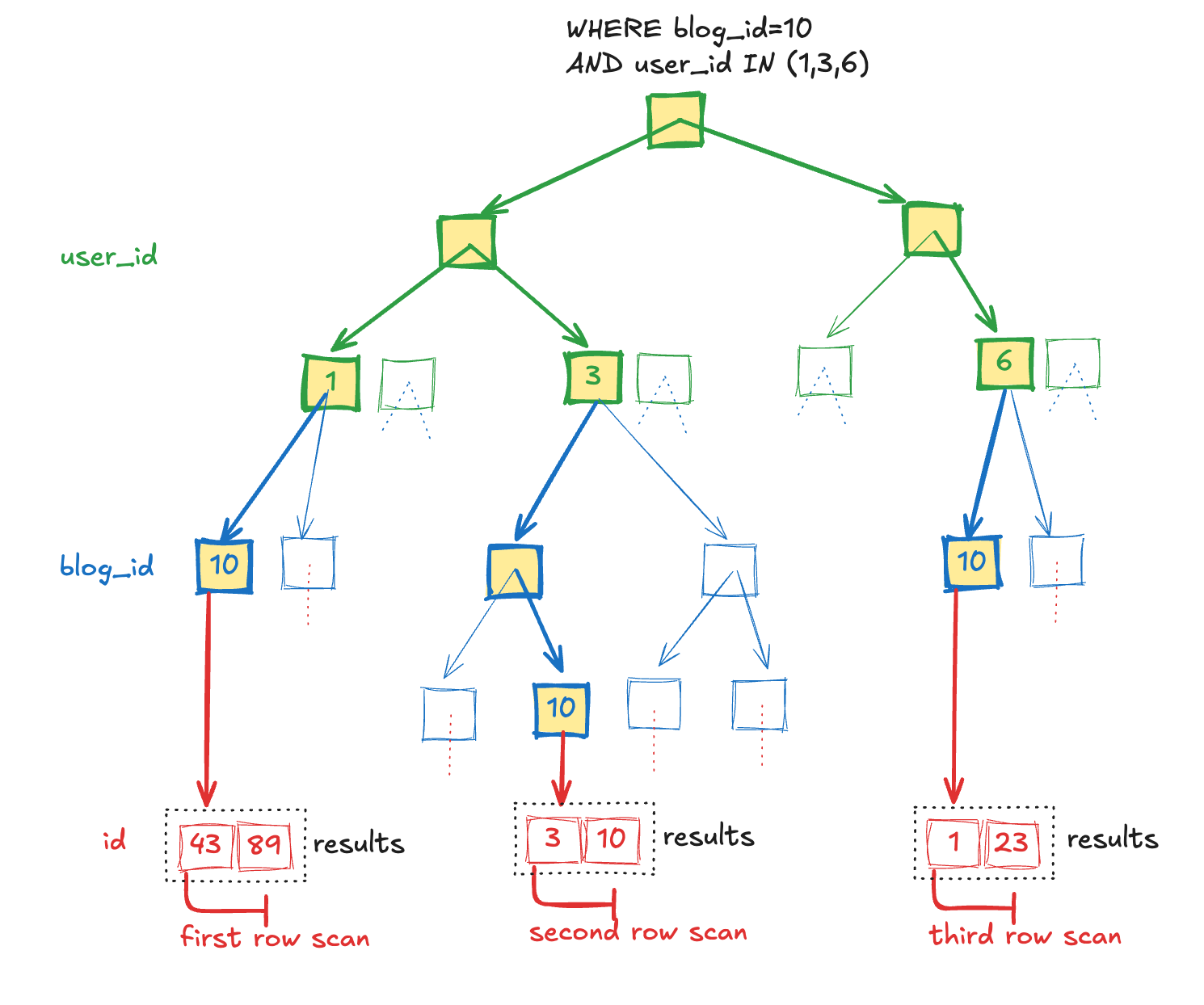
Let’s look at a more concrete example to help explain. Let’s say we have an index on [user_id, blog_id] and want to query for WHERE blog_id=10 AND user_id IN (1,3,6). Mysql is going to break this down and navigate the index three seperate times:
-- first iteration
WHERE blog_id=10 AND user_id=1

-- second iteration
WHERE blog_id=10 AND user_id=3

-- third iteration
WHERE blog_id=10 AND user_id=6
Each of these iterations can be fully solved by the index [user_id, blog_id], just like a ref-type query!
This is true even though we have the range involved column (user_id) in the first position of the index. A finite-range query does not prevent us from using the blog_id portion of the query.
Post-Index Computations
Although Mysql will always start off by using an index if possible to reduce the amount of post-processing required, it goes without saying that not every query will be fully solved by an avilable index. There are a couple post-index computations that we should consider the relative performance of.
First, if the query is requesting an ORDER which differs from how the index sorts its rows, a filesort will be required. This is an expensive operation (O(nlogn)) if the number of rows to be sorted is large. In addition, sorting requires Mysql to temporarily buffer the entire dataset (eg you can’t stream a sorting operation). See ref-type queries for a reminder how indexes naturally sort rows.
If the WHERE clause of the query was not fully solved by the index, Mysql will also need to scan through the rows one after another to apply the remaining filtering. While this is faster than a filesort, it is also relatively slow for large data sets (O(n)). If the index reducing the dataset down to a reasonable size upfront, then this may not be a big deal.
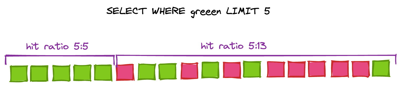
There is one exception here: if the query also specifies a LIMIT x, Mysql need not scan the entire dataset. Mysql will “short circuit” the row scan as soon as it has enough rows to satisfy the query condition. The performance of this kind of pattern is dependent on the “hit ratio” of rows. If there are relatively few rows that satisfy the filter condition compared to rows that must be dropped, then Mysql will need to scan for a longer time compared to if almost all the rows are valid. In addition, you may find that the “density” of interesting rows is not constant throughout the range being scanned! If your application is paginating through a large data set, you may find that different pages have different query times, depending on how many rows need to be filtered out on each page.
Join Algorithms
Nested-Loop Join
The primary algorithm used by Mysql to join tables is a couple variations on “nested-loop”. This a very straightforward algorithm:
for each row in tableA:
  for each matching row in tableB:
    send to output steram
Because Mysql is often capable of streaming joins, when the join query includes a LIMIT x the full join may not have to be executed:
- Mysql executes query in the outer table
- For the first row in the range, look-up matching rows in the inner table
- For each matching row, emit to output stream
- Stop execution if enough rows found, otherwise move to next row and goto 2
Note that similar to un-indexed row scans, this does not apply to all conditions (for example, if sorting is required the full dataset is required in memory).
Hash Join
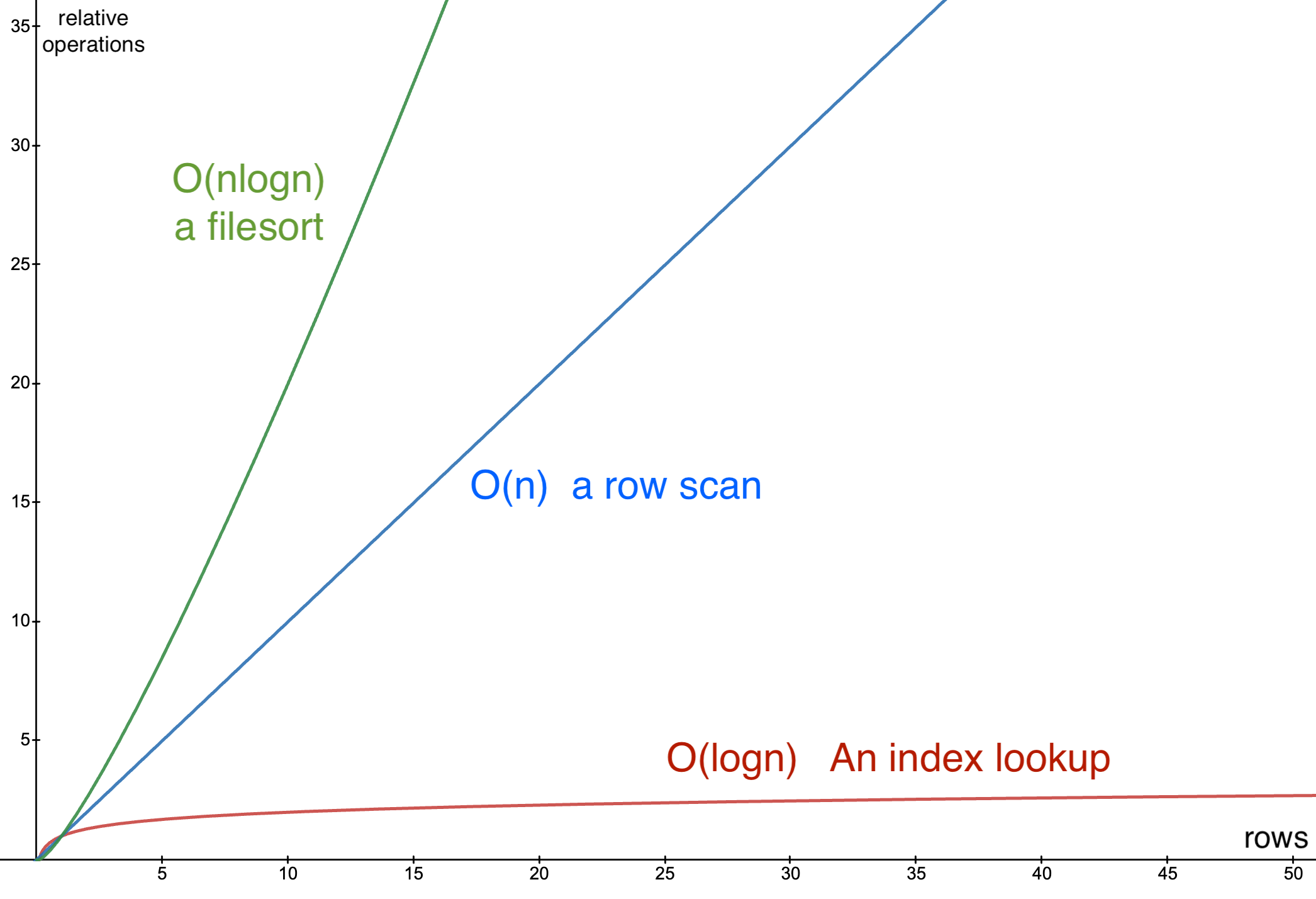
The hash-join algorithm avoids the N+1 B-tree traversal by taking some time upfront (O(n)) to build an in-memory hash table. The reason this strategy can give a performance improvement over nested-loop in some cases is because a hash table lookup has an average profile of O(1) compared to B-tree traversal at O(logn). Given we may have to do this lookup many times (m times), the overall performance profile of hash-join is O(n + m), whereas nested-loop’s profile is O(nlogm).
The below plot shows the region (shaded blue) where the function n+m has a lower value than n*logm:
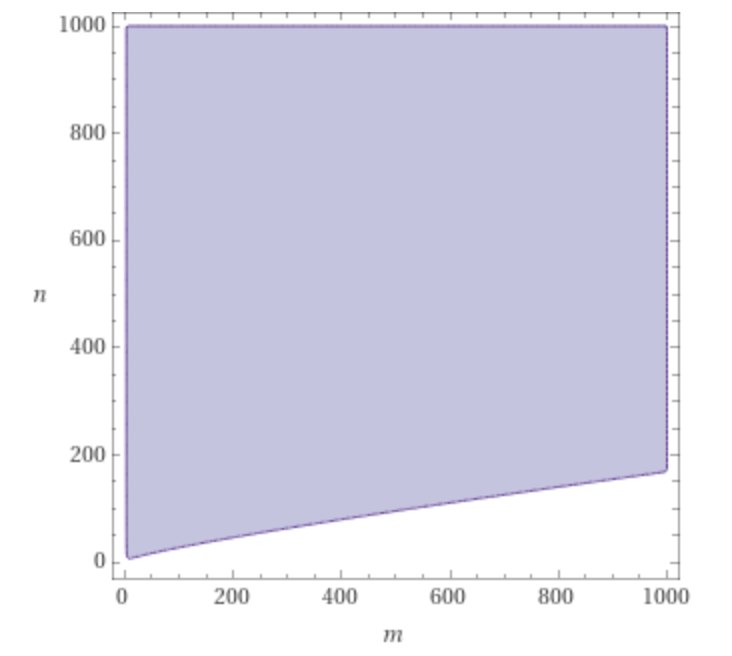
The tradeoff is of course that this (potentially large) hash table must fit into memory. For this reason one strategy to improve hash-join performance is to limit the size of this temporary table by SELECT-ing only those columns which you really need (to reduce width), and pre-filtering as many rows as possible (to reduce height).
The second thing to keep in mind for performance of hash-joins is that indexes on the join condition will not be used. Rather, the place to focus is on indexing any independent filters if possible. For example, consider the following query:
SELECT * FROM tableA t1 JOIN tableB t2
ON t1.shared_id = t2.shared_id
WHERE t1.colA = "foo"
AND t2.colB = "bar"
The best indexes for this query given a hash-join would be on t1.colA and a second index on t2.colB. Execution of this join would then look like:
- Use the index on
colAto find all rows in t1 wherecolA = "foo". - For each row, build a hash table where the key is
t1.shared_idand the value is the row. - Use the index on
colBto find all rows in t2 wherecolB = "bar". - For each row, look up the matching t1 rows from the hash table by
t2.shared_id
Applied Example: Compound Cursor Iteration
Lets take a look at a practical example of how we might apply some of this knowledge.
In this example, we want to iterate through all blog posts that were created since the start of the year. By default, our application is built to use ID-based pagination, and therefore our query has taken the following form:
SELECT * FROM blog_posts
WHERE created_at >= "Jan 1"
AND id > 234890  -- Our pagination cursor
ORDER BY id ASC
LIMIT 1000
In an attempt to optimize this query we have added an index on [created_at, id]. Yet we have found that the performance of this query is still very poor.
Lets take a look at the EXPLAIN format=json for this query as-is (I’ve only included the interesting parts):
{
    "using_filesort": true,
    "table": {
        "table_name": "blog_posts",
        "access_type": "range",
        "possible_keys": [
            "index_created_at_and_id"
        ],
        "key": "index_created_at_and_id",
        "used_key_parts": [
            "created_at"
        ],
    }
}
Looking at the above EXPLAIN there are two major problems:
- Only the
created_atportion of the index is being used (because there are multiple true-range conditions) - The query is using a filesort (because the ORDER BY does not match the used index)
Put another way, the query plan looks something like this:
- Use the index to find the first row created this year
- Scan rows sequentially until we find all the rows with ID above 234890
- Load all these rows into memory, and sort them
- Return the first 1000 rows
Our index is only helping with the first step, not good!
One potential solution to this problem is to switch from a basic ID-based pagination cursor, to a compound cursor. In this case, I will propose a cursor of [created_at, id], which matches the index we have on the database.
Remember, the pagination cursor is just the value of the final row on the most recently loaded batch. For simplicity, lets label the parts of the compound cursor using x & y:
x = previous_batch.last.created_at
y = previous_batch.last.id
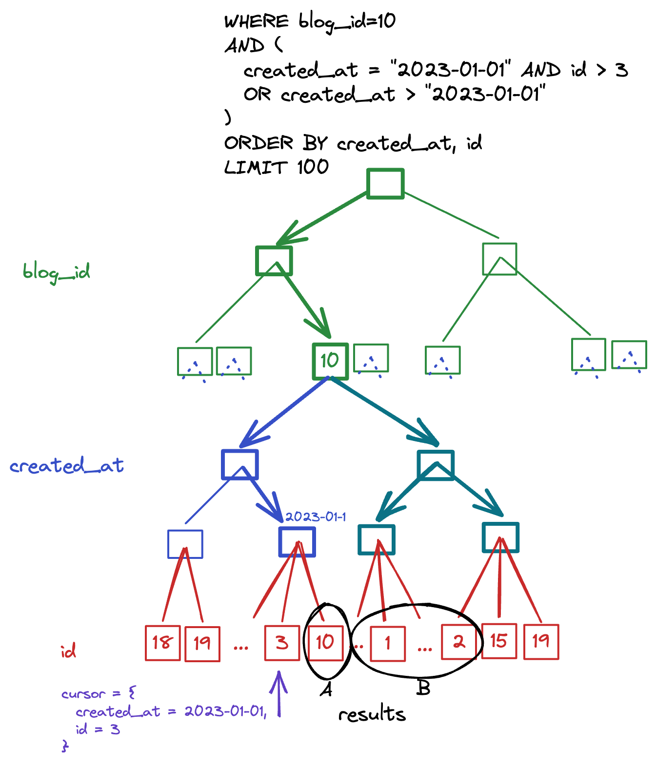
When using a compound pagination cursor, the stucture of the query will look as follows:
SELECT * FROM blog_posts
WHERE
  created_at = x AND id > y
  OR created_at > x
ORDER BY created_at, id ASC
LIMIT 1000
Let’s analysis the above query a bit more closely. As a reminder, the two performance problems we were aiming to fix were:
- The filesort
- The multiple range conditions
First, notice that the ORDER BY clause is now created_at, id. Because this is the natural ordering of our [created_at, id] index, the filesort will no longer be required!
Next, it appears at first glance that this query still has multiple true-range conditions which will still prevent mysql from fully utilizing our index. However, notice that we have also introduced a finite-range condition in the form of an OR clause. Before we jump to any conclusions, lets break the finite-range query down into its parts:
-- Query A: the "left" side of the OR clause
SELECT * FROM blog_posts
WHERE created_at = x AND id > y
ORDER BY created_at, id ASC
LIMIT 1000

-- Query B: the "right" side of the OR clause
SELECT * FROM blog_posts
WHERE created_at > x
ORDER BY created_at, id ASC
LIMIT 1000
By analysing the OR clauses piece-wise like this, we can now see that each index navigation has only one true-range filter. Combining this with the fact that the ORDER BY is the natural ordering of these indexes, we have solved both of the original problems! No more filesort, no more unsolvable double-range filters.
🟡 A note of warning: this pattern may only work as you expect for columns that have immutable values. Like any data structure iteration, if a value changes during your iteration your process may either process a row twice or not at all! For example, consider if instead of iterating on created_at, id we were iterating on updated_at, id. If a row is updated (and therefore updated_at increases) while a process is already iterating through the dataset, we may see that updated row twice: once with its lower updated_at value, and again with the higher value.