Proof of Work Hashrate Equilibrium Maths
Note: this is simply a thought experiment without any real practical use cases. It depends on knowing the cost function of all available hashing power, which is unrealistic (although an approximation may be possible to gather with market research)
This page takes the definitions on Proof of Work Mining Profit Equations as axioms
Equilibrium Marginal Cost
As defined in Proof of Work Mining Profit Equations, \(\alpha\) is the cost per hash at which any new actors who can provide hashes below this rate are incentivized by profit to do so, and any actors whose costs are above this rate are incentivized to leave the market by losses.
Because new actors entering the market in profit lowers the value of \(\alpha\), and there is not an infinite amount of cheap electricity and silicon, we should expect there to be a value \(\alpha^*\) that \(\alpha\) is tending toward; the equilibrium marginal cost.
Let us assume that there is a function \(f(c)\) which is the amount of hashrate available (used or unused) at a given cost per hash. For the purposes of this page we will assume both that we can know this function and that it is unchanging over time. Both these assumptions are unrealistic, but useful for thinking about how the mining system is attempting to reach equilibrium at any given moment.
If we put this function on a plot, we can identify which regions of cost are already being used for mining, and add the point along the x-axis that marks the maximum profitability \(\alpha\).
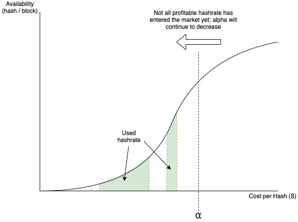
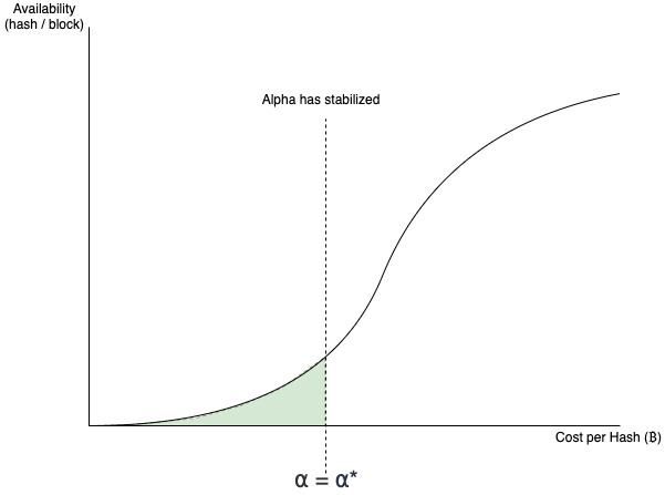
The green shaded area in these plots is the total used hashrate \(H_g\). As more miners enter the market, \(H_g\) necessarily increases, while decreasing \(\alpha\). Eventually, the shaded area becomes “fully compressed”, with no more available profitable hashrate able to enter the market. At this point we can say the market has reached equilibrium, and is also the state at which the maximum global hashrate is being consumed:
\[\alpha = \alpha^*\]
\[H_g = H_g^*\]
Global Total Hashrate
Because the hashrate is “fully compressed” in the above plot when \(\alpha = \alpha^*\), if we knew the value of \(\alpha^*\), we would be able to calculate the total global hashrate consumed by taking the area under the curve:
\[H_g^* = \int_{0}^{\alpha^*} f(c) dc \tag{1} \]
In the following sections, we will work toward deriving \(\alpha^*\).
Global Average Break-even Cost
A vital thing to note is that in this equilibrium state no new miners are able to enter the market, this because the system is at global breakeven. In other words, the total cost of all miners globally is equal to the total block reward \(C_g^* = R_g\)
We also know that the total cost of miners globally would be the average global cost per hash \(\bar{C_g^*}\) multiplied by the total number of hashes \(H_g\). Therefore:
\[R_g = \bar{C_g^*} * H_g \tag{2} \]
Global Average Hash Cost
How do we define the average cost of a hash globally \(\bar{C_g^*}\) ?
One way to think of this value is by taking an average of the continuous cost axis \(x(c)=c\) from 0 to \(\alpha^*\), weighted by how much hashrate is being used at each cost. Using the weighted average of continuous function equation, this gives us:
\[\bar{C_g^*} = {\int_{0}^{\alpha^*} c * f(c) dc \over \int_{0}^{\alpha^*} f(c) dc } \tag{3} \]
Equilibrium Marginal Cost
We now have all the components required to solve for \(\alpha^*\). If we substitute both equations (1) and (3) into equation (2), we are left with:
\[R_g = {\int_{0}^{\alpha^*} c * f(c) dc \over \int_{0}^{\alpha^*} f(c) dc } * \int_{0}^{\alpha^*} f(c) dc \]
Note that the second term cancels out the denominator of the first term, therefore we are left with:
\[R_g = \int_{0}^{\alpha^*} c * f(c) dc \tag{4} \]
Since \(R_g\) is a well known value dependant only on time, and we have assumed that \(f(c)\) is available or can be approximated, it is now possible to solve for \(\alpha^*\). This can in turn be used to solve for the equilibrium total global hashrate via equation (1) above.