Proof of Work Mining Profit Equations

The goal of this note is to define a relationship between miner’s profit and their chosen hash rate, given the externally controlled block reward and global market hash rate.

For the sake of simplicity, we will assume that we are measuring profit per block, and that the miners are fully pool based such that revenue is received on every block. While this is not strictly realistic, it does statistically approximate reality over the long term.

Basic Profit

Let:

• \(h\) be the subject’s desired hash rate (number of hashes per block)
• \(\bar{h}\) be the subject’s current hash rate (this would be 0 for a brand new miner)
• \(c_m\) be the subject’s marginal cost per hash
• \(R_b\) be the current block reward (note: in the same currency as the marginal cost)
• \(H_g\) be the global existing hash rate

In this case, cost can be defined as \(C = h * c_m\)

And revenue can be defined as \(R = {h * R_b \over H_g - \bar{h} + h}\)

Since profit is by definition revenue less costs \(P = R - C\), we arrive with: \[P = {h * R_b \over H_g - \bar{h} + h} - h * c_m\]

Assuming all else is constant, plotting profit (on the y axis) against hash rate (on the x axis) gives a relationship of the form below

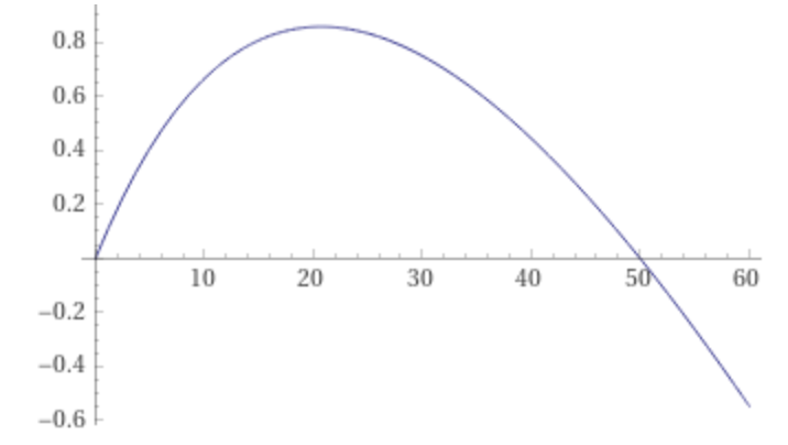
Break-even Hashrate

Using the above profit equation we can derive the maximum hashrate before experiencing a net loss (the x-intercept in the above plot), by setting \(P = 0\) and solving for \(h\):

\[h = {R_b \over c_m} - H_g + \bar{h} \]

Maximum Profit Hashrate

We can determine which hashrate would result in the highest profit for the miner (the apex of the curve in the above plot), by solving for where the first derivative of profit is 0:

\[0 = {dP \over dh} = {R_b * (H_g - \bar{h}) \over (H_g - \bar{h} + h)^2} - c_m\]

\[h = {\pm \sqrt{R_b * H_g * c_m - R_b * c_m * \bar{h} } - c_m * H_g + c_m * \bar{h} \over c_m}\]

Note that we can discard the negative root since negative hash rates do not exist.

Max Marginal Cost to Break-even

In the above profit vs hashrate plot: decreasing the marginal cost \(c_m\) will increase the x-intercept, while increasing marginal cost will decrease the x-intercept and max potential profit until the entire curve is underwater. It is of interest to know at which marginal cost does the curve switch from its up then down mode (ie profit possible), to its only down mode (ie even a single hash is a net loss). We will call this special marginal cost \(\alpha\).

Since the Break-even Hashrate equation above is the x-intercept, we can say that \(\alpha = c_m\) when \(h = 0\):

\[0 = h = {R_b \over \alpha} - H_g + \bar{h} \] \[\alpha = {R_b \over H_g - \bar{h}}\]

Max Marginal Cost over Time

The mining market is not a static thing, the values of \(\alpha\) and \(H_g\) change over time as participants enter and leave the market. We cannot possibly predict what the market actors will choose to do, but we can run some thought experiments about where \(\alpha\) would stabilize given a known or approximated market. This is explored in Proof of Work Hashrate Equilibrium Maths